Pluralis is building Protocol Learning¹. For Protocol Learning to succeed, decentralized training must be competitive with the centralized baseline. Training in a decentralized setting is challenging due to variable node speeds, unreliable connections, and synchronization bottlenecks². This blog post covers our work, Nesterov Method for Asynchronous Pipeline Parallel Optimization (ICML 2025), which eliminates the synchronization bottlenecks, bringing decentralized training closer to the centralized baseline.

Our work shows that asynchronous pipeline parallelism (PP) can surpass the synchronous baseline in large-scale language modelling tasks. By adapting the Nesterov Accelerated Gradient (NAG) to handle gradient staleness³, we achieve stable convergence with 100% pipeline utilization, training up to a 1B parameter model. Furthermore, we demonstrate its effectiveness in decentralized settings with SWARM, again surpassing the synchronous baseline.

Synchronous PP suffers from a bottleneck, where weights and gradients must be synchronized between stages, resulting in idle time known as bubbles (Fig. 1). This idle time is amplified in decentralized settings, where latency is high and bandwidth is low caused by slow nodes and consumer-grade interconnects (e.g. open internet on 80Mbps).

Asynchronous methods remove this bottleneck by overlapping communication and computation (meaning nodes no longer remain idle), effectively masking the communication time between stages. However, as nodes no longer wait for the corresponding backward pass, their gradients become stale, necessitating a delay correction.

We first introduce PP in the naive synchronous setting and highlight its inefficiencies. We then walk through a synchronous pipeline schedule (GPipe) and an asynchronous pipeline schedule (PipeDream) highlighting the gradient staleness issue. Finally, we discuss our Nesterov based look-ahead method that compensates for stale gradients. We prove that our asynchronous PP method converges at a sublinear rate. For full details, including the proof of this convergence, we refer the reader to the full paper. Our code is publicly available here.

Pipeline Parallelism#

Synchronous#

PP splits the model across stages (throughout, the terms node, stage, and GPU are used interchangeably). Fig. 1 below shows a simplified (ignoring communication between GPUs) instance of synchronous PP using 4 GPUs, tracing the forward and backward passes of 2 minibatches. Evidently, utilization is poor, with only a single GPU active at any time. Furthermore, when considering the inter-node communication, the system is limited by the slowest link in the pipeline.

GPipe#

GPipe uses microbatches, which split a minibatch into equal-sized parts, see Fig. 2 below. This improves pipeline utilization, as GPUs can process forward passes of different microbatches in parallel before waiting for their corresponding backward passes. However, all microbatches within a minibatch must use the same model weights, so GPipe performs an optimizer step across all stages at the end of each minibatch, this is known as a pipeline flush. This happens before the next minibatch begins. As we can see there are pipeline bubbles which hinder utilization.

Asynchronous#

We now introduce asynchronous PP, which achieves 100% pipeline utilization in steady state, as shown in Fig. 3 below. Compared to the GPipe example, weights in this setup are updated at every backward step rather than only through a pipeline flush. The key observation is that the weights used for a forward pass may be updated multiple times before the corresponding backward pass for that same microbatch. The side effect of this is stale gradients, where the gradients of the model are computed with respect to outdated model weights and these stale gradients are used to update the current model weights. This creates an optimization challenge that requires a delay correction mechanism to ensure stable convergence.

This staleness in gradients is the number of backward passes that occur between a forward pass and a corresponding backward pass for a stage. Let the number of pipeline stages be \( P \) and, the update schedule be \( K \), then for stage \( i \), the staleness is:

When \( K = 1 \), which means the weights are updated for every microbatch the delay becomes \( \tau_i = P - i \), as shown in Fig. 3. This is known as a One-Forward-One-Backward (1F1B) schedule.

To illustrate the staleness, observe GPU1 in Fig. 3. Microbatch 5 runs its forward pass right after update B1, but by the time its backward pass B5 arrives, B2, B3 and B4 have already updated the weights. As a result, B5's gradients are old compared to the current weights of GPU1. In addition to this staleness in the optimizer update, inconsistent weights between F5 and B5 in GPUs 1, 2 and 3 cause incorrect gradient computation. Specifically, these intermediate stages have updated their weights and therefore the backward pass of B5 would use different weights than what was used for F5. This inconsistency causes incorrect backpropagation ⁴, which needs to be mitigated.

PipeDream#

PipeDream is an asynchronous PP optimization method that ensures correct backpropagation with weight stashing. Specifically, each forward pass is paired with its own cached copy of the weights for use in the backward pass. This ensures synchronous backward passes with asynchronous weight updates. However, it does not correct for gradient staleness: the cached weights correspond to outdated model weights, so the resulting gradients are applied without delay compensation.

Delay Correction with Nesterov Method#

We now introduce a variant of Nesterov Accelerated Gradient (NAG) as a delay correction mechanism. NAG was originally introduced to speed-up convergence in convex optimization via a look-ahead step that anticipates the next update. In this step, a look-ahead point is calculated by extrapolating the previous update in weight space, so the gradient used in the next update is evaluated at this extrapolated point rather than at the original one. We use this extrapolation technique as a mechanism for delay correction. This is shown in Fig. 4 below. By controlling the smoothness of update directions through its momentum term, NAG improves stability in the case of noisy gradients. As a result, delay correction does not make strong assumptions about the loss landscape, outperforming alternatives like gradient forecasting and learning rate discounting.

Compared to original NAG, we introduce gradient discounting (highlighted in blue) to guarantee convergence with stale gradients. The resulting weight update can be written as:

Where \( \gamma_t \) is the momentum coefficient, \( \eta \) is the learning rate, \( d_t \) is the look-ahead, \( \bar{d}_t \) is the delayed look-ahead, \( \nabla f \) is the gradient of the loss with respect to the weights, \( w_t \) is the current weights, and, \( \bar{w}_t \) is the stale weights. To make this more concrete, the algorithm can be described in the following steps:

Tying this back, we can see how the two terms adjust for stale gradients:

• \( w_{t} + d_{t} \) drives the update toward the current momentum trajectory, mitigating the staleness of the future gradient that will be computed at the updated point.
• \(\eta\,(1-\gamma_t)\nabla f\big(\, \bar{w}_t + \bar{d}_t \,\big) \) applies a discounted gradient that was computed at weight \( \bar{w}_t + \bar{d}_t \) due to the look-ahead at a previous update step, where \( \bar{w}_t + \bar{d}_t \) approximates the current weight value \(w_t \).

There are two important points here: firstly, the delayed look-ahead \( \bar{d}_t \) lines up with the delay in weight space over training, meaning that the \( \bar{d}_t \) captures the delay. Second, the discount factor \( \gamma_t \) grows (or set closer to 1) during training. As \( \gamma_t \to 1 \), the gradient term is scaled down to almost nothing, and the update is dominated by the look-ahead \( d_t \). The significance here is that momentum increasingly takes over the update, smoothing the weight trajectory and naturally absorbing the staleness.

Results#

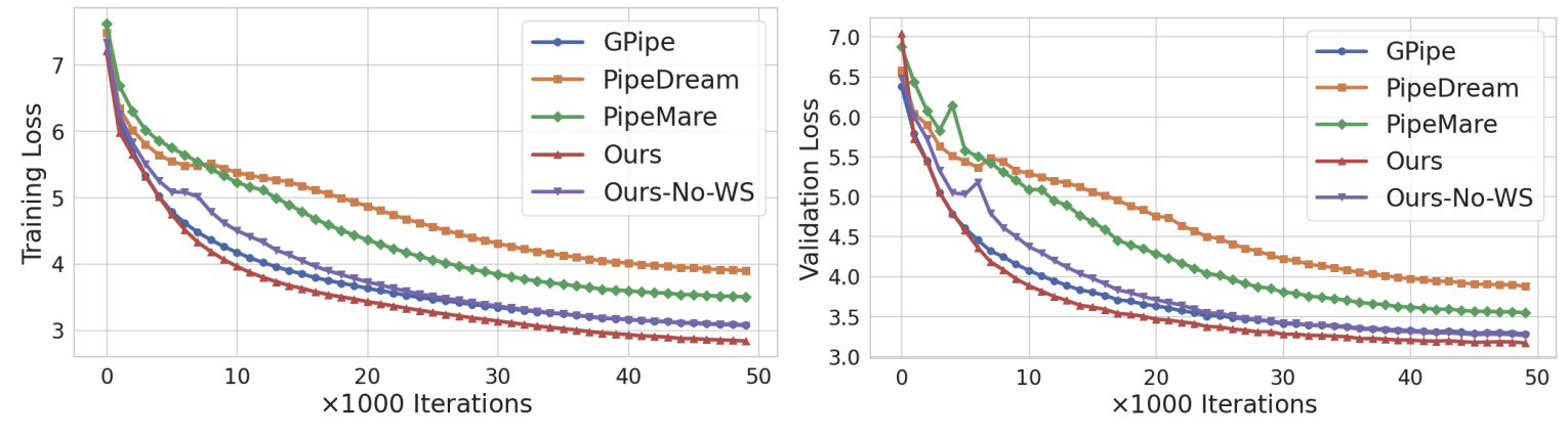
To validate our method for large-scale language modelling tasks, we trained many models, up to a 1B parameter, decoder-only⁵ model was trained within the asynchronous setting. Fig. 5 below compares our NAG-based method against existing scheduling approaches. Our method outperforms all other asynchronous baselines (PipeDream and PipeMare) and, when using weight stashing, outperforms the synchronous GPipe baseline. Even without weight stashing, performance remains competitive with GPipe. These results demonstrate the feasibility of asynchronous PP optimization for large-scale model training and show that gradient staleness can be mitigated without any loss in performance.

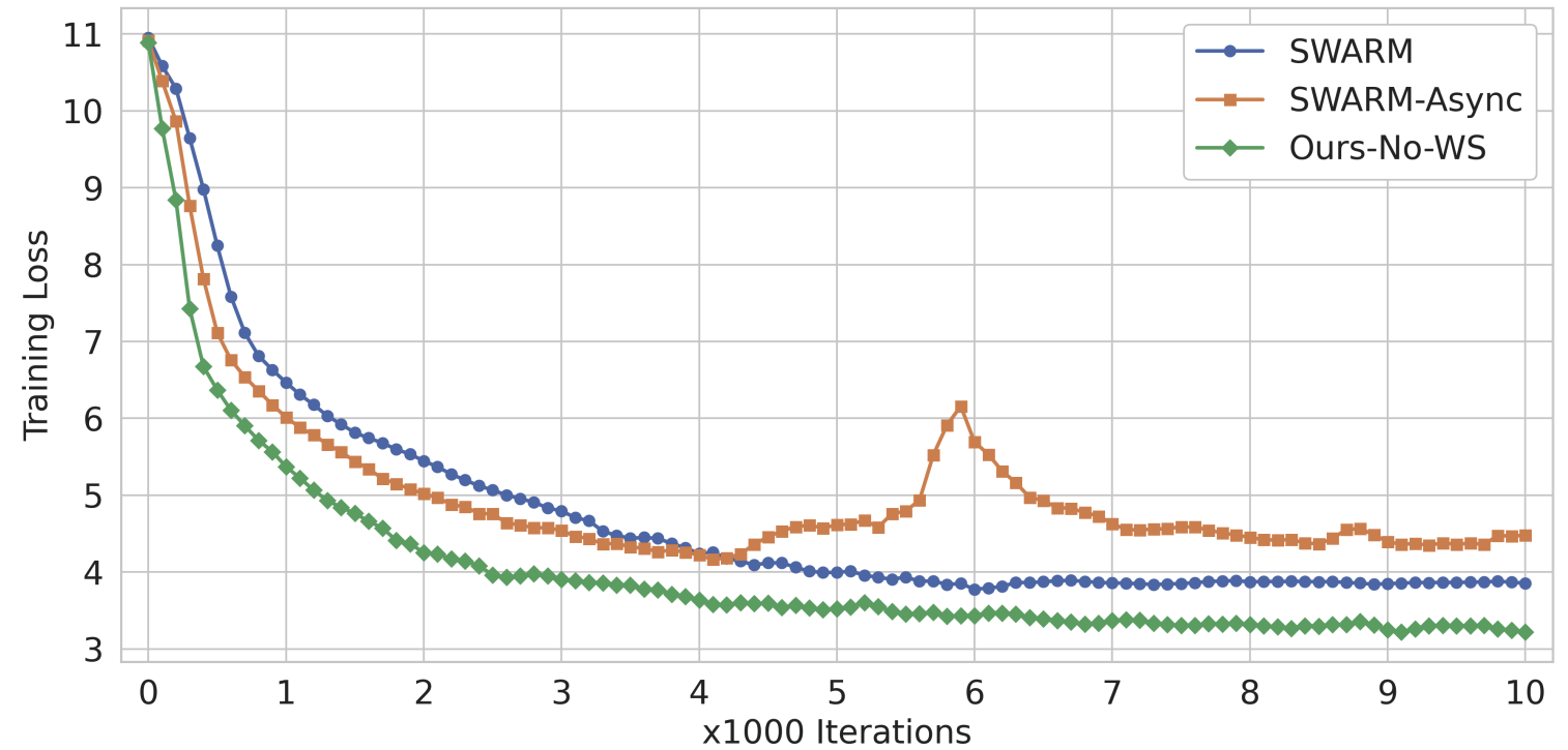
We further evaluate the method in the decentralized regime using a SWARM-like setup⁶, which is built on the Hivemind framework that, which was forked to build Node-0⁷. Fig. 6 below shows that our approach outperforms both SWARM (synchronous) and SWARM-async baselines. This marks the first demonstration of stable asynchronous training in a decentralized model parallel setup framework.

Conclusion#

This post walked through asynchronous PP and its challenges. Our method alleviates stale gradients with a NAG-based delay correction in weight space, using a look-ahead, achieving both high utilization and stable convergence, as well as eliminating bottlenecks. For the first time, asynchronous PP not only matches but surpasses synchronous baselines in both centralized and decentralized regimes. These results are a key step toward towards making decentralized training and Protocol Learning feasible. We refer the interested readers to the paper for more details.

Citation#

For citations, please cite the original paper using the BibTeX citation:

@article{ajanthan2025asyncpp,
  title={Nesterov Method for Asynchronous Pipeline Parallel Optimization},
  author={Ajanthan, Thalaiyasingam and Ramasinghe, Sameera and Zuo, Yan and Avraham, Gil and Long, Alexander},
  journal={ICML},
  year={2025}
}

References#

1. Huang, Y., Cheng, Y., Bapna, A., Firat, O., Chen, M. X., Chen, D., Lee, H., Ngiam, J., Le, Q. V., Wu, Y., & Chen, Z. (2019). GPipe: Efficient Training of Giant Neural Networks using Pipeline Parallelism. arXiv:1811.06965
2. Ryabinin, M., Dettmers, T., Diskin, M., & Borzunov, A. (2023). SWARM Parallelism: Training Large Models Can Be Surprisingly Communication-Efficient. ICML 2023
3. Harlap, A., Narayanan, D., Phanishayee, A., Seshadri, V., Devanur, N., Ganger, G., & Gibbons, P. (2018). PipeDream: Fast and Efficient Pipeline Parallel DNN Training. arXiv:1806.03377
4. Nesterov, Y. (1983). A method for solving the convex programming problem with convergence rate o(1/k^2). Doklady Akademii Nauk SSSR, 269, 543.