Pluralis' Multi-party Training Stack

Pluralis Team

Post authored by James Snewin

January 2026

This post introduces our library built for fault-tolerant, model-parallel, multi-party training over the internet. Training in a collaborative setting at large scale is fundamentally different to how models are trained today. This meant we had to build a novel library that sits at the same layer as DeepSpeed or Megatron-LM, but designed for multi-party training. This library facilitates training in a permissionless distributed system with unreliable nodes, using a mixture of hardware connected by low bandwidth.

Below we will cover the challenges we faced training in a decentralized environment with a production workload. This setting introduces challenges beyond communication alone, such as unreliability and heterogeneity. We will detail the system and research solutions we implemented in our library to address these challenges, which were validated in our public open run, where we trained a 7.5B OLMo-style model trained over the internet with over 1.7k globally distributed consumer-grade GPUs (see hero image above).

Training Environment#

The goal of decentralized training is to leverage geographically distributed consumer-grade compute to train models larger than any one device could do individually. While Pipeline Parallel training paradigms allow us to shard a model's layers over devices and thus fit them onto the VRAM of consumer-grade GPUs, there are several challenges that make this style of training extremely difficult. These challenges stem primarily from the heterogeneity of consumer hardware (different GPU qualities and capabilities), the geographic distribution itself (resulting in low-bandwidth, high-latency connections), the dynamic nature of hardware availability due to pre-emption, and the susceptibility to malicious behavior in a permissionless setting. We summarize these below, and contrast them to the centralized case.

Low Bandwidth#

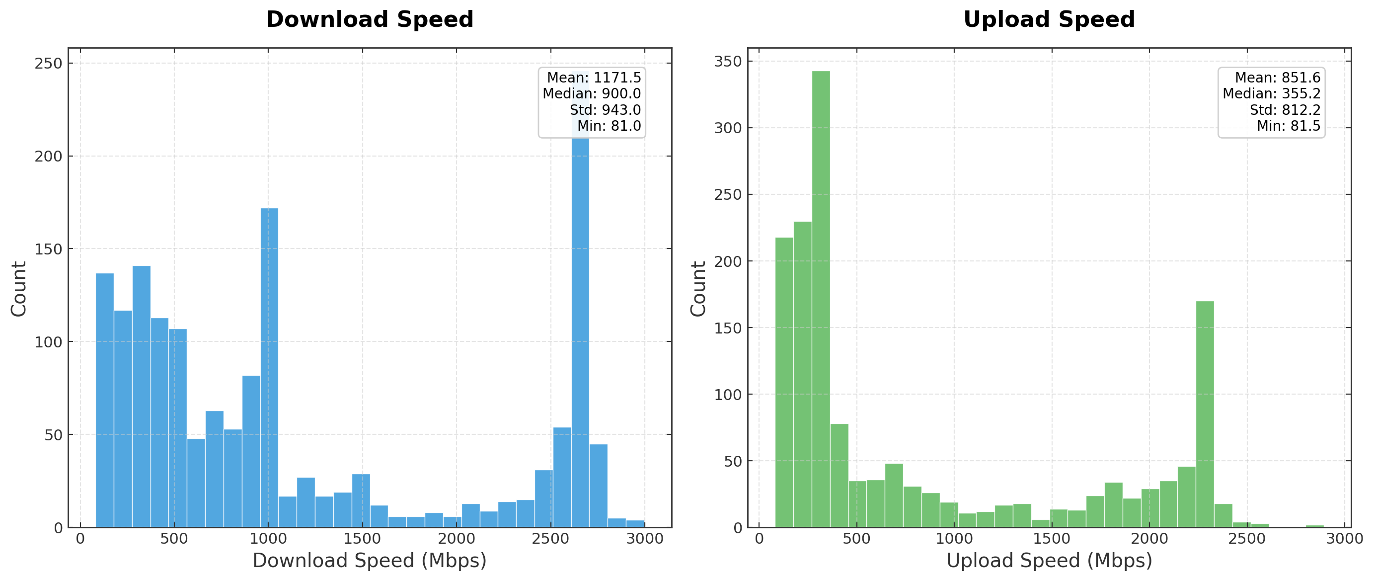
Nodes that are not colocated must communicate via the internet with bandwidth as low as 80Mbps (Fig. 1). This is in contrast to how training is done today inside datacenters where bandwidth can be 100-1000x larger, with Infiniband (100Gb/s inter-node) and NVLink (1TB/s for intra-node) respectively. Moreover, complete control over the communication layer allows tight coupling with the Model Parallel (MP) dimensions. Allowing GPUs within the same rack to leverage Tensor Parallel with NVLink, and Infiniband for Data Parallel (DP).

To make this difference in magnitude more apparent, consider the following example of a forward pass in a Pipeline Parallel (PP) setup: a 7.5B model, 4K embedding dimension with 32 layers, using FP32 and a 4K sequence length. The size of a single activation with a batch size of 1 would be 67MB or 563Mbits. Using 100Mbps, this will take 5 seconds to send, and ~3 minutes across all stages for a single forward pass. With Infiniband this would take 5.6ms per stage and 180ms per forward pass. Crucially, in modern networks, training requires hundreds of thousands of these passes; at internet grade bandwidth this would result in unfeasible training times - evidently, compression is needed in this setting.

Dynamic Hardware Availability#

In standard centralized training, frameworks assume reliable nodes with deterministic communication patterns and phases, and provide basic levels of fault tolerance for faulty devices, greatly simplifying the system design. In a decentralized setting, nodes can frequently drop out at any time during training. The system hence needs to handle constant liveness faults¹ as normal behaviour.

Heterogeneity#

Our library needs to support a large range of hardware, meaning devices differ vastly in FLOPs, memory and latency. A side-effect of this heterogeneity is the straggler effect, where slow nodes can throttle the system, hindering performance. Heterogeneity will cause nodes to process batches at different rates, and averaging algorithms (e.g. nodes doing an all-reduce to average gradients) between them must account for this. For example, in the 7.5B model example above, a T4 would process the batch in ~ 0.25 - 0.35s (~8.1 TFLOPs at FP32) whereas a 3090 would do it in ~ 0.04 - 0.07s (~35.6 TFLOPs at FP32). Centrally, devices and interconnects are homogenous and performance is predictable, removing these effects and simplifying the design.

Adversarial Nodes#

In any system that is open, one must assume the presence of adversarial actors, which will act maliciously to benefit themselves to the detriment of the system. For instance, a worker may produce random gradients that are cheaper for them to produce than correct gradients - these are not conducive to training and could degrade convergence. A weak form of verification is currently used in Node-0, that checks code integrity - eventually this should be extended by adding both byzantine fault-tolerant optimization, and verification at the stage level, or addressed via similar approaches.

Addressing The Challenges#

We address these challenges through both system and research solutions, which correspond to the distributed system layer and the compression layer respectively. Both of these layers are tightly coupled and have unique constraints that directly influence the behaviour of one another - for example, adapting communication primitives for training like all-reduce to work may alter the optimal approach and algorithm to implement DP training at the model level.

The Stack#

The stack is complex, requiring touching several usually disparate areas including Distributed Systems, Distributed Training Algorithms, Machine Learning, and P2P networking. We organize our explanation around key challenges and their solutions. To address dynamic hardware and heterogeneity, we describe the distributed system that enables fault tolerance and dynamic workload orchestration. For low-bandwidth constraints, we detail our compression mechanisms. Finally, we examine the ML challenges that emerged from these solutions. Before diving into these specifics, we establish a mental model of the broader system design by drawing comparisons with existing frameworks.

Existing Frameworks#

To understand the scope of what we're building, we can make comparisons between datacenter based training. Fig. 2 below summarises this; the red outline highlights the training library described in the post.

Starting Point#

The libraries we are replacing in Fig. 2 above are typically maintained by 100s-1000's of volunteer contributors and took many years to reach the state they are in today. We were able to build this because there existed a first pass at many of the problems in the excellent HiveMind library. We also greatly credit the work of SWARM, which provided a strong foundation for the system architecture.

HiveMind gave us:

• A distributed hash table (DHT) acting as a distributed storage layer, based on the Kademlia Protocol that allows for decentralized discovery and redundancy of state.
• P2P fault tolerant communication primitives (all-reduce, all-gather etc.).
• An averaging mechanism to synchronize state between nodes.
• A mixture of experts framework, supporting the sharding of model layers to perform a PP style of training.

HiveMind was critical - without it, we would not have been able to build this library with the limited resources we had. However, we found ourselves running into the limits of the library as we scaled to larger models, modern architectures (HiveMind originally only supported ALBERT), more participants and more realistic training workloads. In the sections below, we will cover what we built on top of this foundation.

Distributed System Layer#

The distributed systems layer is responsible for coordinating training across unreliable, heterogeneous nodes operating over the internet, this can be thought of as the control plane.

Architecture#

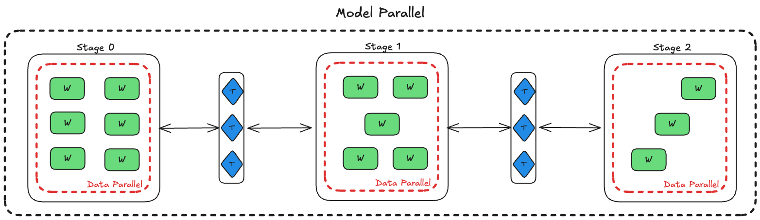
The system is a dynamic, elastic, heterogeneous GPU network, which uses both PP, a special case of MP, and DP. The model is split into stages, where each stage hosts a subset of the layers (Fig. 3). Workers within a stage represent the DP dimension and the number of stages represents the PP dimension. The compute graph of the model is distributed across nodes in this setting.

There are two main roles in the system:

• Workers: GPU-bound workload that is responsible for running and hosting the stage's model layers (think nn.module). These nodes compute forward and backward passes and do gradient synchronization via all-reduce with peers within a stage.
• Trainers: CPU-bound workload that exists outside of stages. Has entire knowledge of the network architecture and stages, and orchestrates the flow of data, sending activation and activation gradients between workers in stages. This can be thought of as a standard pytorch training script where the model is replaced with a set of end-points hosted by workers to send batches to.

Fig. 4 below captures the dynamic between trainers and workers.

We also introduce other roles that are supporting infrastructure and are not part of the core training loop. These are:

• Seeds: these nodes act as boot nodes, serving as an entry point for peer discovery inside the DHT. They are launched before workers and trainers.
• Authorizer: authorizes nodes to participate in the training run.
• Health monitor: scrapes the DHT to aggregate node metrics and stores them.

Fault-tolerant Optimization Protocol#

Our distributed setup operates without central orchestration. Consensus on collective operations (such as all-reduce) must therefore be reached through matchmaking mechanisms² that don't rely on a central decision-making entity. The original HiveMind all-reduce (the underlying primitive used for state updates) implementation used Moshpit SGD. In our setting, we found Moshpit SGD to be unsuitable: it required multiple all-reduce rounds, making it too slow and assumes large group sizes within a stage (e.g. 50-100 nodes), where in practise we would have much fewer (as nodes can drop out at anytime). This caused it to often fail to reliably form groups and average correctly.

To address this, we used a fault-tolerant butterfly all-reduce (which is suitable for a single all-reduce round) that continues processing with the available peers when other peer(s) drop out, producing a partial update rather than failing the round. To illustrate this, consider the following example of nodes within a stage, completing gradient averaging in the DP axis (see Fig. 5 below):

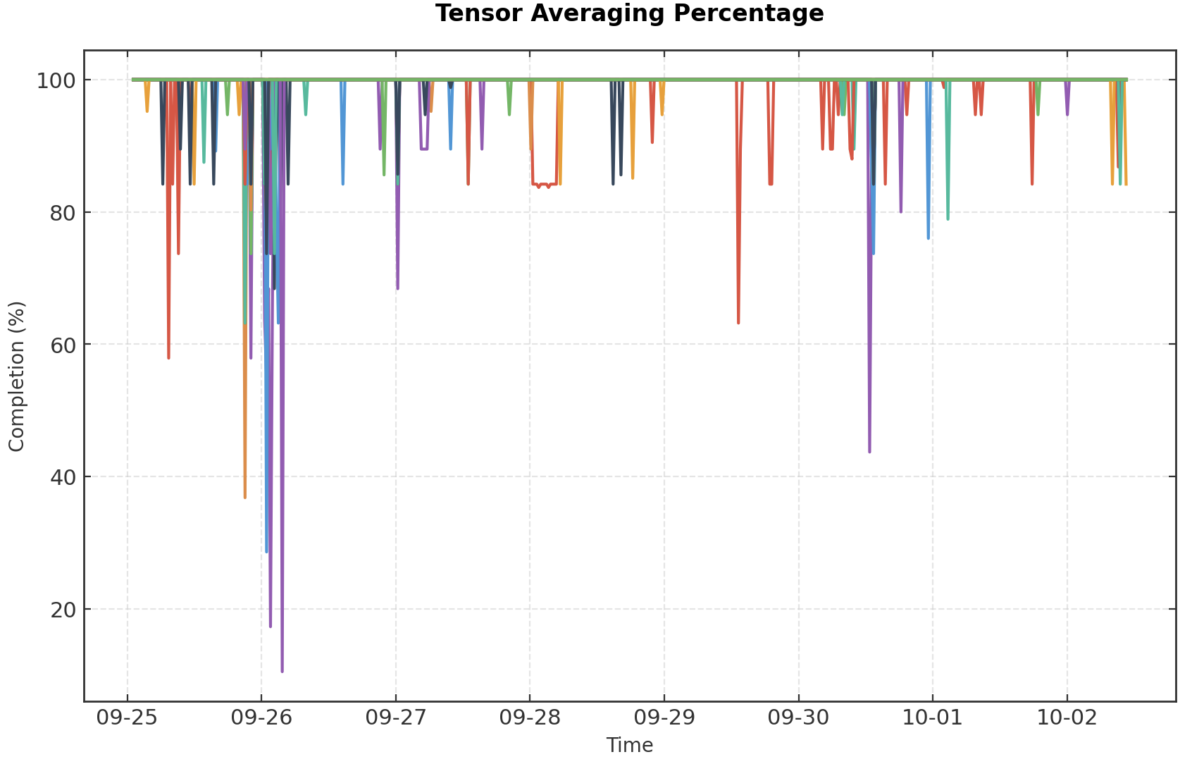
Training must continue gracefully in this scenario. We encountered this frequently during the live run; Fig. 6 below shows the percent of tensors successfully averaged within matchmaking rounds, where 100% represents a successful all-reduce with all peers. In some cases, nodes only could successfully all-reduce with 10% of their peers.

To avoid these pitfalls, we rewrote the matchmaking mechanism and designed a decentralized update procedure we termed the FTOptimizer. The FTOptimizer implements a fault-tolerant state (gradients, weights etc) update (Refer to Appendix A for a code block of this algorithm). The protocol must:

• Orchestrate the node join procedure from acquiring layer state to participating in batch processing (link to state synching section).
• Manage weight drift to prevent bad activation or gradient contributions from nodes that are too slow.
• Dynamically optimize bandwidth utilization by preventing heavy communication overhead at critical points (e.g., avoiding state sharing during all-reduce phases).
• Prevent weight divergence between nodes within a stage due to partial all-reduce failures.
• Enable graceful rollback from old checkpoints (although this wasn't needed during the run) despite iteration counters varying between stages.

Trainer Batch Routing#

Trainers manage a queue of workers to route batches to (Fig. 4), with priority being based on the workers effective throughput, measured by the batch roundtrip time. In the original SWARM implementation, newly joined workers were placed at the head; this is so trainers can gain heuristics quickly on the new workers (such as throughput) - this ended up being problematic. We found that during the run, under heterogeneity, when slow nodes would join and leave frequently the overall system TPS would significantly reduce due to new nodes receiving preferential load. What this meant is that the effectiveness of the trainer's load balancing was reduced, where faster nodes were under utilized. We solved this by inserting new joiners at the bottom of the queue, meaning TPS remained unaffected as fast workers remained prioritised.

Distributed Hash Table Scaling#

The DHT is the entry point and conduit for communication in the network, and as the system scaled to more stages and participants, it quickly became a bottleneck. For example, all nodes across stages would report to, and be discovered, via the same DHT⁵. We handled this by increasing the amount of DHT instances run by trainers – this allowed us to separate the DHTs by stage, meaning any two stages would not share the same cross-stage information, preventing DHT communication bottlenecking the protocol at scale.

Node Joining - and State Staleness#

Nodes joining a stage mid-run must download the layer state (weights and optimizer states) from an existing node with the latest version. Since each layer contains 2.4GB of data, this transfer can be time-consuming. To manage this process, we restrict state sharing to the beginning of batch accumulation rounds (within the first 10% of the round). If the joining node has sufficient bandwidth, it can complete the download and participate in the round with the current layer state. We also permit nodes to join with staleness of up to 5 rounds. If a node cannot complete the state download within this 5-round window, it must rejoin and restart the download process. To handle the potential weight staleness introduced by this procedure, we interleave gradient updates with infrequent sparse parameter state-averaging (see SPARTA section below).

Checkpointing#

Distributed checkpointing is complex especially in the absence of a centralized orchestrator. However, this is a critical feature in order to support mid-run branches, rollbacks, and restarts - both in development and testing and in live runs. We also would like to be able to port checkpoints from the SWARM to centralized frameworks like TorchTitan for fine tuning and evaluation.

In centralized checkpointing, such as in torch.save(), the framework will gather and commit the step count, optimizer state, and weights. However in our system, all of this state information differs per-stage. Because there is no concept of a global state, checkpointing meant we had to stage-wise checkpoint by timestamp instead of by step.

This drift arises because stages progress independently; meaning there is no way to globally coordinate on a time to take a checkpoint. To capture the model state that actually achieved a given loss value, we need to save weights from each stage at the corresponding point in its own iteration timeline (by timestamp), even though these snapshots may be offset. While unconventional, this approach accurately represents the complete model state that produced the observed loss.

Communication Efficient Training#

The compression layer adapts model architectures and training algorithms to operate under low bandwidth. We will introduce these research solutions below:

Subspace Networks#

PP requires high inter-layer communication⁶, making it extremely data hungry, rapidly saturating bandwidth (see the 7.5B example above). In our low-bandwidth setting, this renders training infeasible without activation and activation gradient compression.

To address this constraint, we developed a new class of model architecture known as Subspace Networks (SSN), designed specifically for communication-efficient distributed training. SSNs losslessly compress activation and activation gradients between otherwise unaltered transformer blocks in MP stages, achieving up to a 100x increase in communication efficiency. In this work, we show that this architecture can achieve similar performance at the 8B scale to standard transformer architectures, refer to the paper here for the results. Furthermore, SSNs have been replicated successfully outside of Pluralis at 1B scale, see here.

SSN networks leverage the rank-collapse observed in the projection matrices of large pretrained models (see here and here) and constraints them to a shared and learned low-rank subspace. This reparameterization of the matrices makes the compression lossless. We refer the reader to the original paper here for further details, such as dealing with the high-rank structure from token and positional embeddings, and how the recursive structure of transformers is exploited. Refer to Fig. 7 below that shows this compression for stages in the MP pipeline.

Applying this compression to the previous 7.5B example, with subspace nets, we can compress the activations from 566Mbits to 5Mbits, reducing communication time down 0.05s, a 100x reduction from 5s.

Data Parallel Compression#

Cross-worker communication in the DP axis is required for parameter gradient synchronization before workers do their local optimizer step and is the other potential communication bottleneck. Fortunately, DP compression has been extensively studied in the literature; for example (non-exhaustive) DiLoCo a variant of Federated Averaging for large models, signSGD, DION, and SPARTA.

HiveMind already implemented PowerSGD (PSGD)⁷ with quantization, for compression. However, we encountered issues with the implementation where faulty nodes would incorporate their own error calculation (see the algorithm here for more details) even when all-reduce failed (note the error calculation is performed after all-reducing the P matrix). To prevent this, we added an additional error backup buffer which would only get updated when both all-reduce phases (P and Q matrices) succeeded and would be re-loaded in case of failure.

The PSGD algorithm approximates the larger gradient tensor \((m, n)\) by the product of two smaller matrices \((m, r)\) and \((r, n)\). As a result nodes only need to share \(O((m + n) \cdot r)\) instead of \(O(m \cdot n)\). Referring to the 7.5B example, a single transformer block would be ~800MB, which would greatly slow down communication time for all-reduces. With PowerSGD we can compress this 64x (the ratio we used in the run), resulting in a size of 12.5MB. Furthermore, PSGD also has strong convergence proofs. These factors make it an attractive choice. Refer to the original paper here for more details on the algorithm and formal proofs.

State Averaging#

A side-effect of all-reduce failures, and the load-state staleness for nodes was weight drifting. For example, a node that fails to all-reduce (and thus also fails the optimizer step) during matchmaking in a PowerSGD round, would have weights that are out of sync with respect to its peers within a stage. This is a trade-off we made; as these failures were so frequent we opted for training to continue and accepted weight drifting⁸, as opposed to retrying all-reduces. To combat this we implemented state averaging, specifically SPARTA (sparse parameter averaging). We selected SPARTA to further compress communication between nodes within a stage. We performed a state averaging step once every 5 gradient steps. Averaging was applied to trainable model parameters and additional data like clipping statistics (see section Clipping). We did not average the optimizer state as it adds communication overhead and is generally more robust to divergences as they are slow moving.

Machine Learning Challenges#

Clipping#

Clipping is a stabilisation technique used to prevent gradient blowups that reduce training stability. Clipping strategies typically make use of a global parameter norm and hence require access to the entire model. In our setting nodes which need to implement clipping have local parameters only and accessing all parameters would require extensive communication. We initially experimented with Zclip⁹ as it was adaptive, allowing us to implement stage-wise clipping with no knowledge of the global norm, however, we found that if a gradient blow-up occurred it took a long time for the EMA to re-adjust, degrading convergence. We hence made the choice to adopt stage-wise clipping methods. This approach is also beginning to be adopted centrally and appears in some recent methods such as Muon.

We set the per-stage clipping to be \(1 / \sqrt{\text{num\_stages}}\) and the tail clipping value to be \(5 / \sqrt{\text{num\_stages}}\); these values were derived empirically to approximate global clipping, adjusted for the parameter count in each group. We conducted several central experimental runs to evaluate their effectiveness and found they had no effect on convergence.

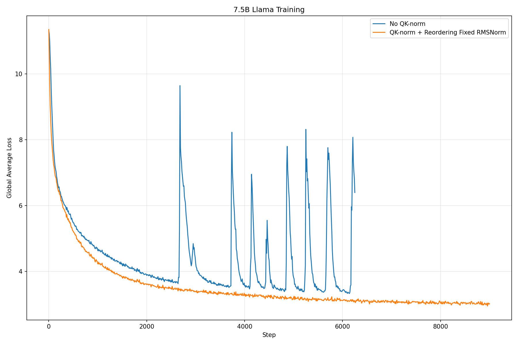
Subspace Networks and Architectural Stability#

When we first integrated SSNs into LLama, we noticed that recovery was slower from loss spikes. We do not know if the addition of SSNs principally was the reason for the divergence relative to the Llama baseline; notably, loss spikes were already reported in the Llama training runs. However, this divergence was present in our Llama + SSN experiments, which prompted further investigation.

We experimented with different techniques such as sophisticated clipping mechanisms and z-loss but eventually implemented QK-norm and re-ordering¹⁰ (which is also implemented within the OLMo2 architecture which was used for the run), which resolved the issue (Fig. 8).

However, the introduction of QK-norm and re-ordering caused the lossless property of SSN compression to break.

The reason re-ordering was not compatible with SSN compression is that SSNs require the output of the transformer block to be in a common subspace with all other blocks. This is due to the residual connection composing these outputs and hence if they are not in a common space, outputs rapidly become uncompressable, destroying information and altering training dynamics. As RMSNorm¹¹ acts element-wise and is therefore nonlinear when the RMSNorm becomes the final operation in the block, we cannot guarantee the final output is restricted to a common subspace. Fortunately, we can easily resolve this by freezing the RMSNorm's trainable element-wise scaling parameters to a single constant value. In this case the operator becomes linear, preserving the recursive structure and allowing the compression to remain lossless after reordering and normalization. In our centralized ablations, we observed freezing the scaling parameters had little to no effect.

Production Training Run#

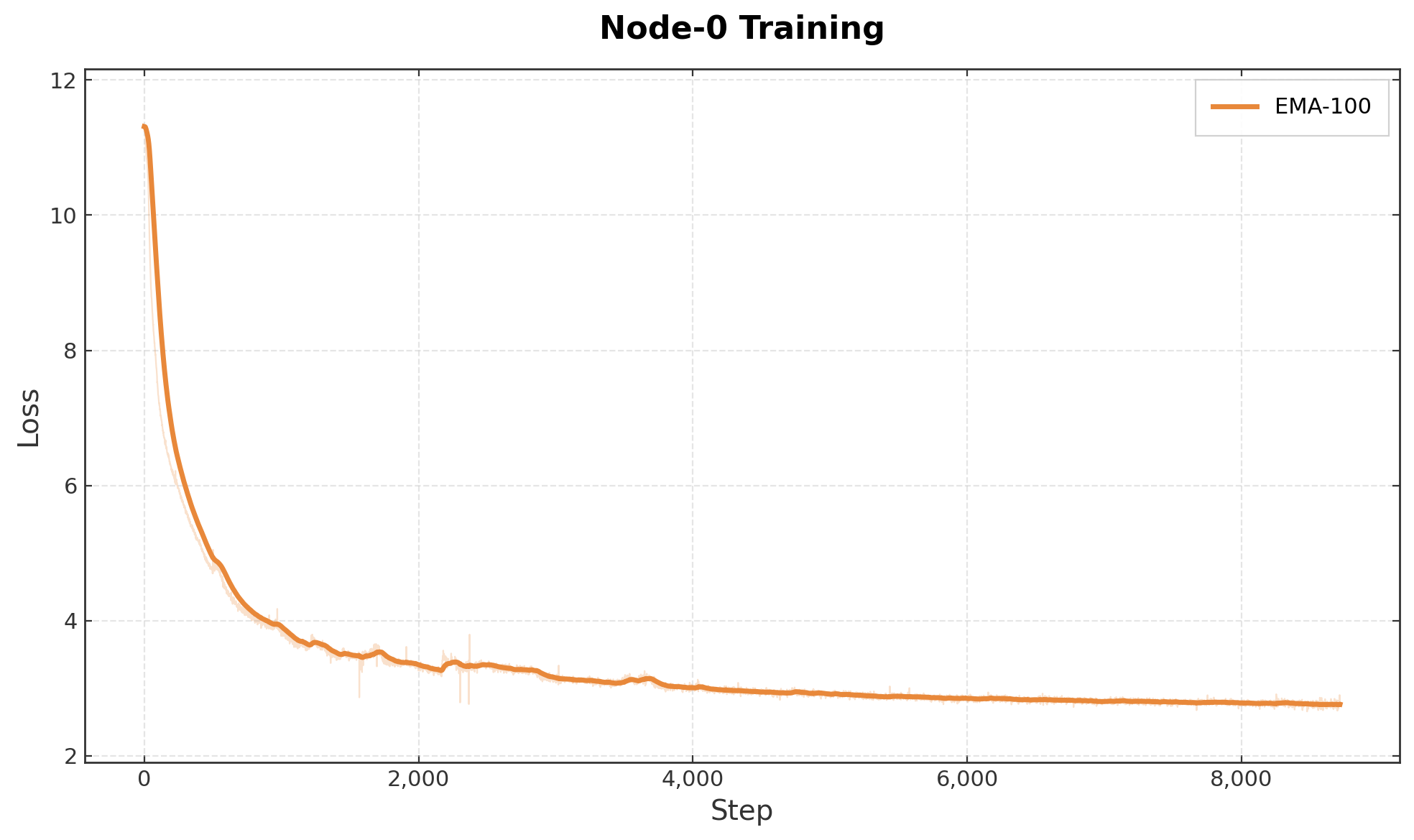
The sections above describe a system designed to operate over unreliable nodes, bandwidth constraints, and heterogeneous devices. To test the system, we conducted a public training run using the full system described above, training a 7.5B OLMo-style model entirely over the internet with globally distributed consumer GPUs. The run went for over 3 weeks and consumed 36B tokens using the fineweb-edu dataset. Through training, the loss decayed down to 2.75 (Fig. 9), tracking a centralized baseline. In total, there were 303 active participants, many of which contributed with bandwidth less than 100Mbps. 78 of the participants contributed more than exoFLOP each.

Conclusion#

This post walked through the design and implementation of our training stack. Because we're building in a completely new setting, many of the challenges we run into like stage-wise clipping aren't covered by existing research. The solutions we describe here come directly from that experience and help push decentralized training forward.

Node-0 is the v0.0.1, and we have a long way to go until decentralized training is competitive with the centralized alternative. But we have shown that this style of training is possible. Valuable insights were gained from this and have major improvements to make in future runs, for example adding asynchronous training¹², making the joining queue a better experience, handling heterogeneity better, and refining our eviction strategies (nodes were evicted if they failed two consecutive all-reduces).

Citation#

For citations, please cite the codebase using the BibTeX citation:

@misc{avraham2025node0,
  title = {Node0: Model Parallel Training over the Internet with Protocol Models},
  author = {Gil Avraham and Yan Zuo and Violetta Shevchenko and Hadi Mohaghegh Dolatabadi and Thalaiyasingam Ajanthan and Sameera Ramasinghe and Chamin Hewa Koneputugodage and Alexander Long},
  year = {2025},
  url = {https://github.com/PluralisResearch/node0}
}

References#

1. Ryabinin, M. & Gusev, A. (2020). Towards Crowdsourced Training of Large Neural Networks using Decentralized Mixture-of-Experts. NeurIPS 2020
2. Beton, M., Reed, M., Howes, S., Cheema, A., & Baioumy, M. (2025). Improving the Efficiency of Distributed Training using Sparse Parameter Averaging. MCDC @ ICLR 2025
3. Ramasinghe, S., Ajanthan, T., Avraham, G., Zuo, Y., & Long, A. (2025). Protocol Models: Scaling Decentralized Training with Communication-Efficient Model Parallelism. arXiv:2506.01260
4. He, J., Li, X., Yu, D., Zhang, H., Kulkarni, J., Lee, Y. T., Backurs, A., Yu, N., & Bian, J. (2023). Exploring the Limits of Differentially Private Deep Learning with Group-wise Clipping. ICLR 2023
5. Kumar, A., Owen, L., Chowdhury, N. R., & Güra, F. (2025). ZClip: Adaptive Spike Mitigation for LLM Pre-Training. arXiv:2504.02507
6. Ryabinin, M., Borzunov, A., Diskin, M., Gusev, A., Mazur, D., Plokhotnyuk, V., Bukhtiyarov, A., Samygin, P., Sinitsin, A., & Chumachenko, A. (2020). Hivemind: Decentralized Deep Learning in PyTorch. GitHub
7. Maymounkov, P. & Mazières, D. (2002). Kademlia: A Peer-to-Peer Information System Based on the XOR Metric. IPTPS 2002
8. Vogels, T., Karimireddy, S. P., & Jaggi, M. (2019). PowerSGD: Practical Low-Rank Gradient Compression for Distributed Optimization. NeurIPS 2019
9. Cho, M., Finkler, U., Kumar, S., Kung, D., Saxena, V., & Sreedhar, D. (2021). PowerSGD: Convergence of Low-Rank Gradient Approximation for Distributed Optimization. arXiv:2102.12092
10. Sharma, P. & Kaplan, J. (2022). A Neural Scaling Law from the Dimension of the Data Manifold. arXiv:2206.08257
11. Martin, C. H. & Mahoney, M. W. (2018). Implicit Self-Regularization in Deep Neural Networks: Evidence from Random Matrix Theory and Implications for Learning. arXiv:1812.04754
12. Ryabinin, M., Gorbunov, E., Plokhotnyuk, V., & Pekhimenko, G. (2021). Moshpit SGD: Communication-Efficient Decentralized Training on Heterogeneous Unreliable Devices. NeurIPS 2021
13. Douillard, A., Feng, Q., Rusu, A. A., Chhaparia, R., Donchev, Y., Kuncoro, A., Ranzato, M., Szlam, A., & Shen, J. (2023). DiLoCo: Distributed Low-Communication Training of Language Models. arXiv:2311.08105
14. McMahan, H. B., Moore, E., Ramage, D., Hampson, S., & Agüera y Arcas, B. (2017). Communication-Efficient Learning of Deep Networks from Decentralized Data. AISTATS 2017
15. Ahn, K., Xu, B., Abreu, N., Fan, Y., Magakyan, G., Sharma, P., Zhan, Z., & Langford, J. (2025). Dion: Distributed Orthonormalized Updates. arXiv:2504.05295
16. Bernstein, J., Wang, Y.-X., Azizzadenesheli, K., & Anandkumar, A. (2018). signSGD: Compressed Optimisation for Non-Convex Problems. arXiv:1802.04434

Appendix#

Appendix A#

# Worker Batch Processing & Gradient Sync Algorithm

# INITIALIZATION
local_epoch, accumulated_samples = 0
weights, optimizer_states = init_weights()
local var max_allowed_stale, target_batch_size, refresh_period
local var average_state_freq
sync var global_samples_accumulated, global_epoch

# INITIAL WEIGHT LOADING (wait for optimal join point)
def load_state_from_peers(wait_for_end_round):
    
    # PHASE 1: WAIT FOR START OF NEW ROUND
    # Only join when peers are at the beginning of a round (< 10% progress)    
    while True:
        if (global_samples_accumulated < target_batch_size * 0.1):
            # Peers are at start of round, safe to join
            break
        else:            
            # Waiting for peers to finish step
            sleep(refresh_period)
    
    # PHASE 2: DOWNLOAD STATE FROM PEERS
    # Download model weights, optimizer states from peers
    weights, optimizer_states = _load_state_from_peers()  
    
    # PHASE 3: WAIT FOR CONFIRMATION OF NEW ROUND
    if wait_for_end_round:
        # Extra safety: wait until absolutely sure new round has started
        while True:
            if (global_samples_accumulated < target_batch_size * 0.2):
                # Confirmed: new round started (< 20% progress)
                break
            else:
                # Downloaded state, waiting for start of new round
                sleep(refresh_period)
    
# Call initial load
load_state_from_peers(wait_for_end_round=True)


# MAIN TRAINING LOOP
while training:
        
    if local_epoch < global_epoch:
        # Slightly behind, catch up epoch counter (allow staleness)
        local_epoch = global_epoch
    
    # 2. PROCESS LOCAL BATCH
    loss, operation = forward_backward_pass(_get_batch_from_queue())
    if operation == "forward":
        continue
    
    accumulate_grads(batch_size, loss.backwards())
    report_progress(local_epoch, accumulated_samples)
        
    # 3. PERFORM GLOBAL UPDATE (if conditions met)
    if global_samples_accumulated >= target_batch_size:
        disable_state_sharing()  # Prevent interference during AllReduce
        
        # Perform matchmaking for upcoming averaging round
        trigger_matchmaking()

        # Perform distributed gradient averaging (PowerSGD)
        average_gradients_with_peers()

        # Apply optimizer step with averaged gradients
        optimizer_step()

        # Perform SPARTA state averaging
        if global_epoch % average_state_freq == 0:
            average_states_with_peers()
                                
        enable_state_sharing()